Manual
Contents
1. What is LocalMove
2. Typical usage scenario
3. In depth description
3.1. Method
3.2. Lattices
3.3. Local moves
3.4. Quality measure
3.5. Simulated annealing
3.6. Initial conformation
3.7. Stopping conditions
4. Web server options
1. What is LocalMove
LocalMove is a webserver dedicated to predicting the best on-lattice fit for biopolymers. Through a sequence of local moves, e.g. local backbone modifications, it walks through the conformational space, looking for a configuration as close as possible to the input 3D model, while keeping his points on-lattice. After a user-defined condition is triggered, the experiment stops and the currently best model can be retrieved as a PDB file.
2. Typical usage scenario
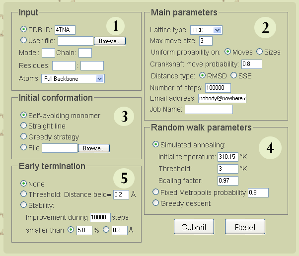
Parameters input page
Set the options and parameters of the simulation and hit the submit button.
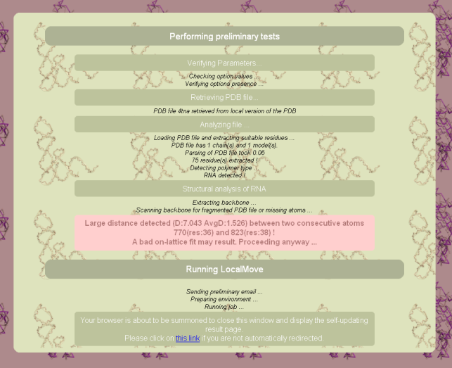
Pre-processing page
A pre-processing page will pop-up or just open as a tab, depending on your browser. It might feature warnings with concern to missing atoms. You should then be redirected to the following realtime progress page:
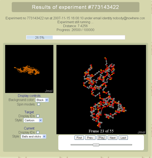
Progress page
This self-refreshing page displays the progress of the ongoing simulation. Namely, it shows the number of steps already performed, the current distance to the original for the best on lattice candidate. Additionally it features both the original model and its current best on-lattice approximation, using the JMol applet. Finally, it is possible to animate the on-lattice model to reproduce the evolution from the initial conformation to the best on-lattice fit so far.
When the simulation is over, you should be redirected instantly to the result page:
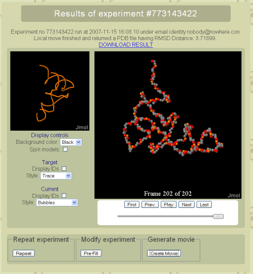
Results page
On the final result page, it is possible to download the best on-lattice fit found during the simulation. A visualization of the model, along with a JMol animated applet which allows to visualize the conformational exploration process. From this page, the whole simulation can be re-run as is, or pre-loaded in the webserver form. An MPEG movie of the exploration process can be computed and retrieved (This feature requires quite some computational ressources, and could take up to several hours for large models).
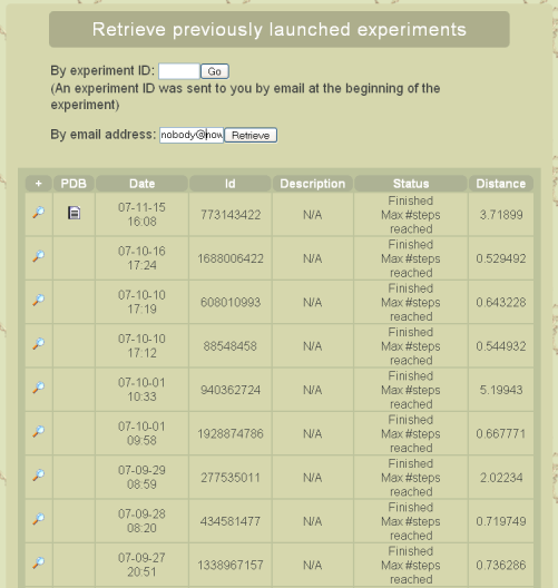
Results retrieval page
Leaving the website through closing your browser do not affect ongoing simulations. However you will need the experiment ID, sent to you by email, to access your results through the Results tab of the website, once your original browser has been closed. If you have lost this information, it is possible to get an history of previous and ongoing simulation for your email address. Please notice that, due to storage limitation issues, simulation results will be deleted after a variable period of time (typically a couple of weeks). If you try to access results for a deleted experiment, you will be proposed to reproduce your experiment, for which you won’t have to re-enter parameters
3. In depth description
3.1. Method. LocalMove performs a Monte-Carlo exploration of the conformational landscape. At each step, a custom Root Mean Square Deviation is computed, which captures the similarity between the current model and the input model. This similarity is then used to compute the probability of accepting the current conformation as the basis for the next move. Additionally, simulated annealing, which simulates the cooling down of a thermodynamical system, can be performed in order to increase the conformational coverage. After several iterations of the system, the most promising conformation is returned to the user.
3.2. Lattices. As of version 1.0 , three type of lattices are currently supported:
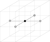 | 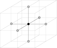 | 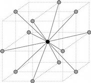 |
| Square lattice | Cubic lattice | Face centered cubic lattice |
Neighbors of a point under various lattice models
- Square lattice (2D) A simple bi-dimensional lattice whose points are
those of the 2D grid on the XY plane. Alternatively, the square lattice can
be defined as the set of points {(x,y,0) | x,y

 }.
}.
- Cubic lattice (3D) This lattice is implicitly defined by the three vectors (1,0,0), (0,1,0) and (0,0,1). Therefore, its points are those of the 3D grid having integral coordinates.
- Face Centered Cubic lattice (3D) This 3D lattice is very similar to the
cubic lattice on even coordinates, except that additional points are added
at the center of every face. As a consequence, the neighbors of a given point
p = (x,y,z) are all points p′ = (x′,y′,z′)≠p reached through two unit steps,
or more formally such that
 +
+  +
+  = 2.
= 2.
3.3. Local moves. The best on-lattice fit search is performed through a sequence of local moves. Local moves are moves that only concern a small subset of atoms and do not affect the rest of the structure. Thus, a local move is the substitution of a self avoiding walk on the appropriate lattice by another self avoiding walk of the same size, having the same relative between its extremities. The relevant parameters handled by LocalMove for such moves are the local move size and the strategy for picking a new local move at random.
3.4. Quality measure. The Root Mean Square deviation (RMSD) between the original polymer and the best superimposed version of its proposed on-lattice version is standardly used to assess the quality of an on-lattice fit. However, this measure would require us to compute, for each of our candidate, the best solid rotation/translation, which would be catastrophic in term of the huge amount of computational ressources required.
Therefore, we define and use a slightly modified version of the RMSD, the RMSDd, which is the root mean square deviation computed according to distance matrices. More specifically, this quantity will capture the divergence between the interatomic distances in both original and candidate models. Our Monte Carlo simulation will aim at minimizing this quantity, which is very close to the real RMSD and can be computed in reasonable time.
It can be proven that this quality measure is rotation-independent, which means that if three models M, N and N* are such that N* is a rotated version of N, then RMSDd(M,N) = RMSDd(M,N*). As a consequence, the only reason why a best predicted model could only be a suboptimal would be because of a translation. This is a significant improvement over previous works, which had to either explicitly or implicitly fix a translation/rotation beforehand.
3.5. Simulated annealing. Simulated annealing is classically used for optimization problems in order for the walk to converge with probability one to the optimal solution. In our case, a pseudo-temperature has an influence over the probability of accepting a move that would temporarily increase the RMSDd (Metropolis steps), but might allow for the walk to escape from a local minimum. Theoretically, this ensures the convergence to a Boltzmann distribution under certain additional properties of the underlying Markov chain.
3.6. Initial conformation. Three strategies are implemented in LocalMove to choose an initial configuration:
- Random: A random 3D self avoiding walk is generated
- Straight line
- Rounded (greedy): After normalizing the polymer such that interatomic distance is 1 on the average on its backbone, we set the starting point to be the closest integral point to the original model, and extend the initial conformation by incrementally adding points that are the closest to that of the original model.
3.7. Stopping conditions. Our Monte-Carlo simulations can be stopped for some of the different following reasons: Either a limit temperature is bypassed during the simulated annealing; a distance threshold is reached; the maximal number of steps have been performed; or the simulation is stalled for too long, leaving few hope for improvement. In the latter, the required improvement over a user-defined period of time can be either relative or absolute.
4. Web server options

- Input parameters:
- PDB ID: The access PDB code for the desired polymer. The file will be retrieved from the PDB if not available locally.
- User file: A user file, formatted according to the PDB file format specifications.
- Model: In NMR data, several models can be present, representing either different snapshots of the molecule or different candidates for the real structure. The user can specify which model to be used for the simulation, otherwise the first model in the specified file is used.
- Chain: A PDB file typically consists of a set of chains of potentially different nature (RNA, Protein, DNA ...), this option allow the user to specify which chain to use. By default, the first chain present in the PDB file will be used.
- Residues: It is possible to restrict the simulation to a consecutive subset of atoms from the input chain. For instance, this allow one to find best on-lattice fit for a specific helix. By default, all atoms from the selected chain are accepted.
- Atoms: Another way to restrict those atoms taken into consideration for the experiment is to focus on the backbone only, or even a restriction of the atoms backbone. Here, available options include all atoms, full backbone(default), C1’/Cα carbons, phosphoruses, Glyc bonds Nitrogens or centers of mass of each residue.
- Main parameters:
- Lattice type: The lattice type to be used for the simulation, chosen among: Square, Cubic or Face Centered Cubic lattice (FCC).
- Max move size: The maximal size for a local move, e.g. the number of nucleotides on which the local structural mutation is performed. Shorter local moves are still allowed, but potentially very unlikely depending on the move size distribution.
- Uniform probabilities: The next local conformation in a local move can either be chosen uniformly among the set of all moves preserving the extremities of the previous local conformation (Value moves), or a size k less or equal to the maximal move size can be chosen first prior to generating a local configuration having size k (Value sizes). The latter biases the generation toward choosing smaller local moves, otherwise neglected due to the exponential growth of the number of local moves on their size, and potentially useful to the fine-tuning of the best candidate.
- Crankshaft move probability: The probability that a move occurs in the inner part of the monomer, as opposed to its extremities. Setting this probability to a low value would facilitate the initial collapse when starting from a straight line initial configuration. However, high values ensures a quicker convergence toward a good on-lattice candidate.
- Distance type: The distance notion used to assess the quality of a candidate. In addition to the RMSDd, it is possible to use the SSE Sum of Squared Errors, which allows for a quicker computation of a distance essentially similar to the RMSDd.
- Number of steps: The number of attempted local moves in the Monte-Carlo simulation. As of version 1.0 the maximal number of steps is 100 000.
- Email address: An email address where the simulation termination notification and experiment id are going to be sent. This field must be filled out.
- Job name: A user defined name for the experiment.
- Initial conformation:
- Self avoiding monomer: A simple self-avoiding walk in the 3D space, taking on-lattice unit steps.
- Straight line
- Greedy strategy: The model built through always choosing the closest position to that of the original model.
- File: A user-defined initial conformation, whose points are already on-lattice, can be input.
- Random walk parameters:
- Simulated annealing: In this mode, the probability of rejecting a bad move (Metropolis step) is proportional to the temperature. An initial temperature is initially used and, each 1000 steps, a scaling factor is applied to the current temperature, until a threshold is bypassed.
- Fixed Metropolis Probability: The probability of accepting a local move that increases distance to the original model (Metropolis step) can be made constant.
- Greedy descent: Local moves that do not improve over the previous on lattice model are always rejected.
- Early termination:
- None: No termination condition additionally to the max number of steps and the simulated annealing temperature threshold.
- Threshold (Fixed): Simulation stops if the chosen distance is below a desired value.
- Stability: Terminates the simulation if the simulation is stalled, and the best on-lattice fit do not improve over a defined period of time (default: 10 000 steps). The required improvement can either be relative (given as a percentage of the previous value) or absolute.