|
How to run BTW?
|
You have three choices:
- Compare your data versus pre-compiled public gene expression time series.
- Compare your data versus itself.
- Compare two different datasets
|
|
Algorithms
|
|
Two algorithms for dynamic time warping are available: the
Clote algorithm (described in a forthcoming paper in the Journal of
Mathematical Biology) and our implementation (and expansion) of the Aach
algorithm (described here). The algorithms are similar but subtly different.
We are currently investigating the correlation between time warping
distances computed by the two algorithms. In general, if a pair of genes
has small time warping distance as computed by one algorithm, it would have
small time warping distance as computed by the other algorithm, but the
overall ranking may be different.
|
|
Input format
|
Your data must have a specific format (here is an example):
- the input file must be a text file organized in columns, tab separated (if your data is an excel file, you can easily convert it to a
tab-separated text file by clicking on "File", then "Save as", and choosing tab-separated text file in "File type").
- the first line contains the time points, starting from the second column; the first column is ignored. Time points should be in minutes.
- all the following rows must contain the gene expression values (either raw, log, normalized, etc.), with no missing data.
If one value is missing, there are methods to obtain a reasonable guess - for example interpolation, splines, etc. - but this is up to you!
Missing values will generate errors or incorrect results.
|
|
Mode 1
|
|
The data that you upload will be compared to one pre-compiled public dataset of your choice, selected from the drop-down menu.
The complete list of available datasets is here.
Since these datasets are usually very large, containing thousands of genes, there is a limit to the data that you can upload: 10 genes.
If your file contains more than 10 time series, you will get an error message.
|
|
Mode 2
|
|
All the gene expression time series (max 100) in the file that you upload will be compared one against each other. Usually,
this kind of analysis is done using distance functions like Pearson's correlation coefficient or Euclidean distance, since in this
case the number of time points of the two analyzed time series is the same. Nevertheless, there are indications that time warping distance
can be a better indicator of similarity even when the number of time points is identical.
|
|
Mode 3
|
|
Here you are requested to upload two files
(max 100 time series each). Then, all gene expression time series in the first
file are time warped against all the series in the second one.
|
|
Parameters
|
A few parameters can be set by the user:
- The experiment(s) name
- The number of time warping distance that will be printed on screen in the output (max 100)
- The time scaling factor - time intervals may be scaled opportunely if the difference between datasets is significant
- The parameter p for the computation of the Sakoe-Chiba band, such that
only pairs of time points which satisfy |i-j*n/m| < (p*n) are considered, where i and j are indexes
running on two time
series of size n and m, respectively. The value of p ranges from 0.3 to 1
(values smaller than 0.3 may cause instability, because the band is too
small).
- Up to three temperature values, used for the computation of the
Boltzmann's pair probabilities (default values are 0.1, 0.5, 1.0).
|
Output
|
The complete output can be downloaded in a gzip-compressed format.
The top ranking gene pairs are presented in a table. You can see a
graphical depiction of the alignment, or the alignment Boltzmann's pair probabilities,
clicking on the respective buttons. The following is an example of alignment
graph:
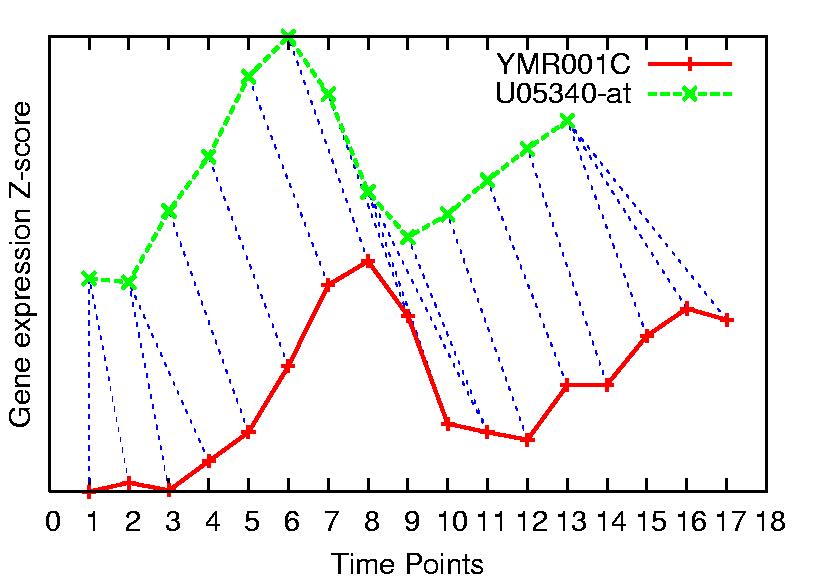
Here two time series are drawn, artificially separated on the gene
expression values axis in order to obtain a clearer description of the alignment.
Aligned time points are joined by a blue dotted line. Note how the number of
points is different, and the major peaks are not aligned on the x-axis.
Thus, these two time series would not result similar using a point-to-point
measure (as Euclidean, Manhattan or Pearson distance).
The following is a Boltzmann pair probabilities graph:
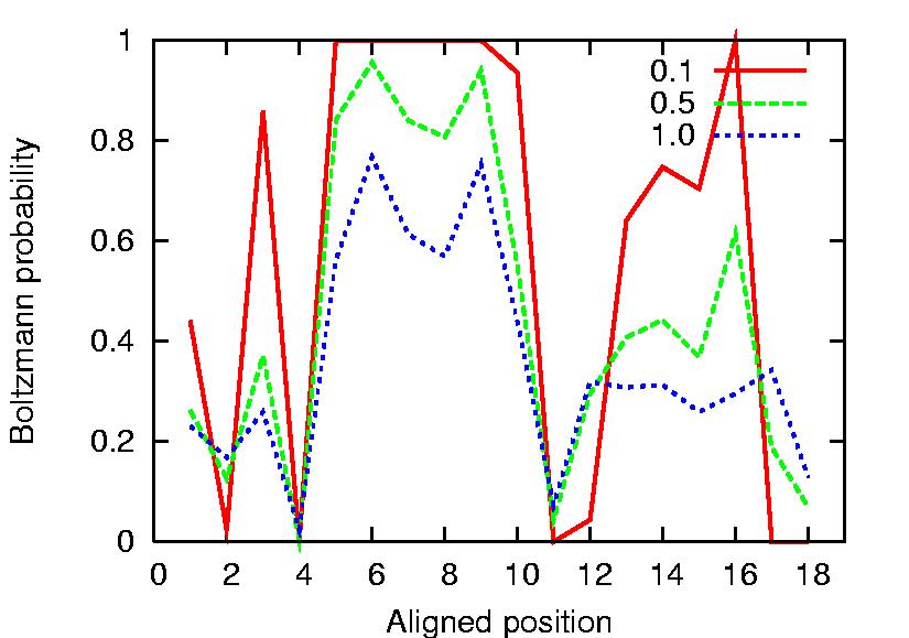
Here Boltzmann probabilities are computed at three different temperatures
:0.1, 0.5, 1.0. Please note that the temperature parameter has not a physical
meaning. You can indicate different T values. Note how the probability of
the alignment points can be remarkably different. This may reflect a higher
alignment accuracy, and may have a biological meaning (for example, high
probability positions can correspond to tighter controlled points during the
cell cycle).
If your favourites gene pairs are not in the top ranking positions,
there is a text box in which you can write it (the format is: geneName[space]geneName - all gene pairs on different lines).
After clicking "submit" you will retrieve the time series alignment and pair probabilities for each selected gene pair. A graph of
the pair probabilities can be visualized or downloaded in eps format.
|
|
|


